What is DBSCAN Clustering in Machine Learning? A Complete In-Depth Guide
Clustering is one of the most powerful unsupervised learning techniques in machine learning. It helps uncover hidden patterns, structures, and relationships in data without relying on labeled outputs. Among the many clustering algorithms available today, DBSCAN (Density-Based Spatial Clustering of Applications with Noise) stands out as a highly practical and intelligent approach, especially when dealing with real-world data that is messy, irregular, and filled with noise.
Table Of Content
- Understanding DBSCAN Intuitively
- Core Concepts Behind DBSCAN
- Epsilon (ε): The Neighborhood Radius
- MinPts: Minimum Density Requirement
- Types of Points in DBSCAN
- How DBSCAN Works Step by Step
- Why DBSCAN is Different from Traditional Clustering
- Strengths of DBSCAN
- Limitations of DBSCAN
- Choosing the Right Parameters
- Real-World Applications of DBSCAN
- Python Example: DBSCAN in Action
- When Should You Use DBSCAN?
- Conclusion
- Related Reads
Unlike algorithms such as K-Means that assume clusters are spherical and require you to predefine the number of clusters, DBSCAN Clustering in Machine Learning takes a completely different approach. It focuses on the concept of density—grouping points that are closely packed together while isolating those that lie in sparse regions. This makes it incredibly useful in domains like anomaly detection, geospatial analysis, and pattern recognition.
Understanding DBSCAN Intuitively
At its core, DBSCAN is based on a simple but powerful idea:
clusters are areas of high density separated by areas of low density.
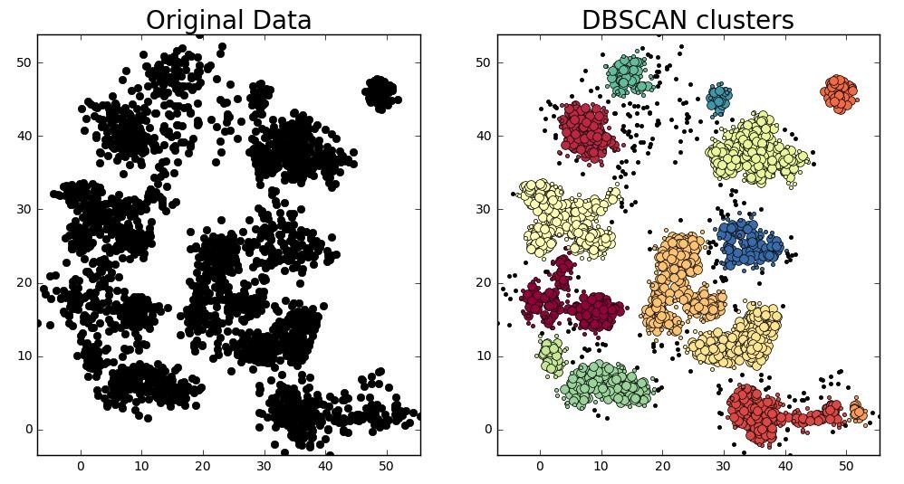
Imagine a map filled with scattered points. Some regions have many points tightly packed together, while others are sparse or nearly empty. DBSCAN identifies the dense regions as clusters and treats isolated points as noise or outliers.
This density-based perspective allows DBSCAN to discover clusters of any shape, unlike traditional methods that struggle with non-linear boundaries.
Core Concepts Behind DBSCAN
To truly understand DBSCAN, you need to grasp how it defines density and connectivity. The algorithm relies on two parameters that control how clusters are formed.
Epsilon (ε): The Neighborhood Radius
Epsilon defines how far the algorithm should look around a point to find its neighbors. If ε is too small, many points will be considered isolated, leading to excessive noise. If it is too large, distinct clusters may merge into one.
Choosing ε is therefore a balancing act. It directly influences how “tight” or “loose” clusters appear.
MinPts: Minimum Density Requirement
MinPts determines the minimum number of points required within an ε-radius to consider a region dense. This parameter ensures that clusters are not formed from just a few random points.
In practice, MinPts is often chosen based on the dimensionality of the dataset. A higher value makes the algorithm stricter, while a lower value allows more flexible clustering.
Types of Points in DBSCAN
DBSCAN categorizes each data point into one of three types based on its neighborhood:
- A core point lies in a dense region and has enough neighboring points within ε
- A border point lies near a dense region but does not have enough neighbors itself
- A noise point lies in a sparse region and does not belong to any cluster
These classifications help DBSCAN build clusters organically rather than forcing assignments.
How DBSCAN Works Step by Step
The working of DBSCAN can be understood as an exploration process across the dataset.
The algorithm begins by selecting an arbitrary unvisited point. It then checks how many points fall within its ε-neighborhood. If the number meets or exceeds the MinPts threshold, the point is labeled as a core point and a new cluster begins to form.
From this starting point, DBSCAN expands the cluster by recursively visiting all neighboring points. If those neighbors are also core points, their neighbors are added as well. This creates a chain reaction that grows the cluster outward through dense regions.
If a point does not meet the density requirement, it is temporarily marked as noise. However, it may later become part of a cluster if it falls within the neighborhood of a core point.
This process continues until all points in the dataset have been visited, resulting in a set of clusters and some remaining noise points.
Why DBSCAN is Different from Traditional Clustering
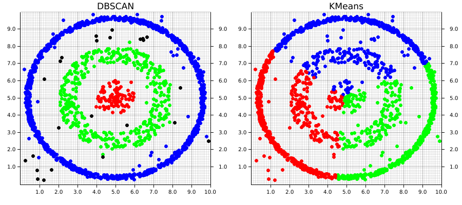
Traditional clustering methods like K-Means rely heavily on distance from centroids and assume that clusters are convex or spherical in shape. This assumption rarely holds true in real-world datasets.
DBSCAN, on the other hand, does not rely on centroids. Instead, it builds clusters based on density connectivity. This allows it to detect curved, elongated, or irregularly shaped clusters that other algorithms fail to capture.
Another key difference is that DBSCAN explicitly identifies noise. While most clustering algorithms force every point into a cluster, DBSCAN recognizes that some data points simply do not belong anywhere meaningful.
Strengths of DBSCAN
One of the biggest strengths of DBSCAN is its ability to work without prior knowledge of the number of clusters. This makes it extremely useful when exploring new datasets.
It is also highly effective at detecting outliers. In many applications, such as fraud detection or network security, identifying anomalies is just as important as finding clusters.
Additionally, DBSCAN performs well with spatial data. Whether it is geographic coordinates, sensor data, or image pixels, the algorithm can naturally group nearby points into meaningful structures.
Perhaps most importantly, DBSCAN can detect clusters of arbitrary shapes. This gives it a major advantage over methods that rely on geometric assumptions.
Limitations of DBSCAN
Despite its advantages, DBSCAN is not without challenges. The biggest difficulty lies in choosing appropriate values for ε and MinPts. Poor parameter selection can lead to either fragmented clusters or overly merged ones.
Another limitation is its sensitivity to varying densities. If one cluster is very dense and another is sparse, a single ε value may not work well for both. This can result in missing clusters or incorrectly labeling points as noise.
High-dimensional data also poses challenges. As dimensionality increases, the concept of distance becomes less meaningful, which can reduce the effectiveness of density-based methods.
Choosing the Right Parameters
Selecting good parameters is crucial for getting the best results from DBSCAN. One common technique is the k-distance graph, which helps identify a suitable ε value by plotting distances to the k-th nearest neighbor.
MinPts is often set based on the number of dimensions in the dataset. A common rule of thumb is to use a value slightly higher than the number of dimensions.
Data preprocessing also plays an important role. Normalizing or scaling features ensures that distance calculations are meaningful and consistent.
Real-World Applications of DBSCAN
DBSCAN has found its way into a wide range of industries due to its flexibility and robustness.
In finance, it is used to detect fraudulent transactions by identifying unusual patterns. In marketing, it helps segment customers based on behavior without predefined categories.
Geographic information systems rely heavily on DBSCAN to group nearby locations, such as identifying hotspots in traffic or crime data. In image processing, the algorithm helps segment objects and detect patterns within visual data.
Autonomous vehicles and robotics also use DBSCAN to cluster sensor data, enabling machines to identify obstacles and navigate safely.
Python Example: DBSCAN in Action
Below is a simple example demonstrating how DBSCAN can be applied using Python and Scikit-learn:
<span class="ͼv">from</span> <span class="ͼ11">sklearn</span><span class="ͼv">.</span><span class="ͼ11">cluster</span> <span class="ͼv">import</span> <span class="ͼ11">DBSCAN</span>
<span class="ͼv">from</span> <span class="ͼ11">sklearn</span><span class="ͼv">.</span><span class="ͼ11">datasets</span> <span class="ͼv">import</span> <span class="ͼ11">make_moons</span>
<span class="ͼv">import</span> <span class="ͼ11">matplotlib</span><span class="ͼv">.</span><span class="ͼ11">pyplot</span> <span class="ͼv">as</span> <span class="ͼ11">plt</span>
<span class="ͼt"># Generate sample dataset</span>
<span class="ͼ11">X</span>, <span class="ͼ11">_</span> <span class="ͼv">=</span> <span class="ͼ11">make_moons</span>(<span class="ͼ11">n_samples</span><span class="ͼv">=</span><span class="ͼy">300</span>, <span class="ͼ11">noise</span><span class="ͼv">=</span><span class="ͼy">0.05</span>)
<span class="ͼt"># Apply DBSCAN</span>
<span class="ͼ11">model</span> <span class="ͼv">=</span> <span class="ͼ11">DBSCAN</span>(<span class="ͼ11">eps</span><span class="ͼv">=</span><span class="ͼy">0.2</span>, <span class="ͼ11">min_samples</span><span class="ͼv">=</span><span class="ͼy">5</span>)
<span class="ͼ11">labels</span> <span class="ͼv">=</span> <span class="ͼ11">model</span><span class="ͼv">.</span>fit_predict(<span class="ͼ11">X</span>)
<span class="ͼt"># Visualize clusters</span>
<span class="ͼ11">plt</span><span class="ͼv">.</span>scatter(<span class="ͼ11">X</span>[:, <span class="ͼy">0</span>], <span class="ͼ11">X</span>[:, <span class="ͼy">1</span>], <span class="ͼ11">c</span><span class="ͼv">=</span><span class="ͼ11">labels</span>)
<span class="ͼ11">plt</span><span class="ͼv">.</span>title(<span class="ͼz">"DBSCAN Clustering Example"</span>)
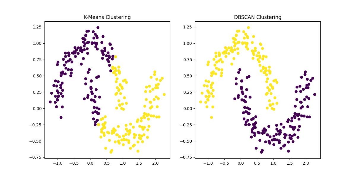
<span class="ͼ11">plt</span><span class="ͼv">.</span>show()This example shows how DBSCAN can easily identify non-linear cluster shapes that would be difficult for algorithms like K-Means.
When Should You Use DBSCAN?
DBSCAN is particularly useful when the structure of the data is unknown and when clusters are expected to have irregular shapes. It is also a strong choice when the dataset contains noise or outliers that should not be forced into clusters.
However, if your data has widely varying densities or exists in very high-dimensional space, you may need to consider alternative approaches or extensions of DBSCAN.
Conclusion
DBSCAN is a powerful and versatile clustering algorithm that offers a fresh perspective on how data can be grouped. By focusing on density rather than distance to a centroid, it overcomes many limitations of traditional clustering methods.
Its ability to discover arbitrarily shaped clusters and identify noise makes it an essential tool in the machine learning toolkit. While it requires careful parameter tuning, the insights it provides are often more realistic and meaningful for real-world data.
As datasets continue to grow in complexity, algorithms like DBSCAN will remain highly relevant for uncovering patterns that are not immediately visible.
Kaashiv Infotech Offers Machine Learning Course, Artificial Intelligence Course, Python Course, Visit Our Website www.kaashivinfotech.com.

